Progressive Income Taxation

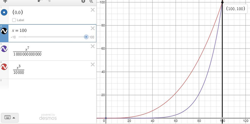
Imagine a graph of income and taxation. The x-axis is labelled annual income, and the y-axis is labelled amount in dollars. The first curve is income, y=x, with a slope of 1. The second curve is ideal taxation. How much of each dollar earned by an American household should be given away in taxes?

At low incomes, households need all of their money, which goes to necessities like food, housing, and transportation. At this interval, income should not be taxed at all. Perhaps there could even be a negative income tax. However, let's say there is a 0% bottom marginal income tax. That means that my amount and rate of taxation approaches 0 as income approaches 0.

At middle incomes, taxation should still be low. Households need some of that higher income to put towards retirement savings or college-education trusts, but can afford some taxation.

At some point, there is an income that is more than what a household needs to afford their current standard of life and their projected length of retirement. That household may spend that extra money of purely discretionary income on restaurant food or vacation, but as they get more and more extra money, they become more likely to invest it. From there, the household will likely reinvest earnings or dividends, essentially blocking money from reentering the American economy. Of course, some money escapes that investor's grasp through commissions or expense ratios, but that invested money is largely gone. At high incomes like these where a dollar earned does not mean a dollar spent and respent within the economy, taxation should be approach 100%.

I immediately backed off that idea of 100% taxation. There would be no incentive to earn money past the lower bound of that bracket, so I arbitrarily chose a top marginal tax rate of 90%.

Actually constructing a function T(x) showing the ideal amount of taxation of dollars was somewhat difficult. I knew what I wanted its derivative R(x), a function of tax rates, to look like:

R(x)=T`(x)

R(x)=0

x->0

and

R(x)=90%

x->infinity

*The little mark (`) by the capital T means the first derivative.

From those limits, I realized R(x) must be a logistic growth function like this:

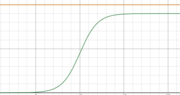
The green line is tax rate, which functions in accordance with the aforementioned limits. The orange line is percent of income kept before tax; it is always 100%.

Therefore, I chose this form:

R(x)= a

1+e^(b-x)

where a is the top marginal tax rate and b is the annual income at which a household can afford all necessities and their retirement.

For my graph, I chose 90% for a and 10 for b (obviously, $10 per year is completely unrealistic).

To get T(x), I simply integrated R(x). Here are the results:

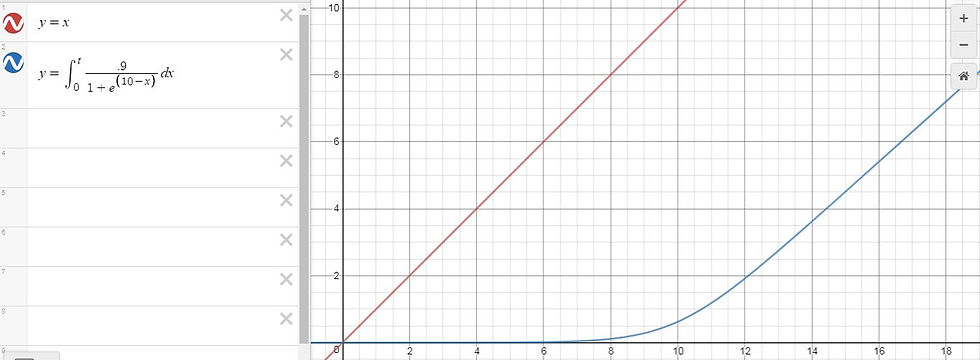
Remember that the x-axis is annual income per household and the y-axis is amount in dollars. As incomes grow smaller, households can keep nearly all of their earnings with a nearly $0 tax amount.

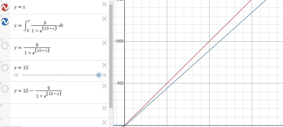
As incomes grow larger, tax amount grows nearly as quickly as income, though not quite:

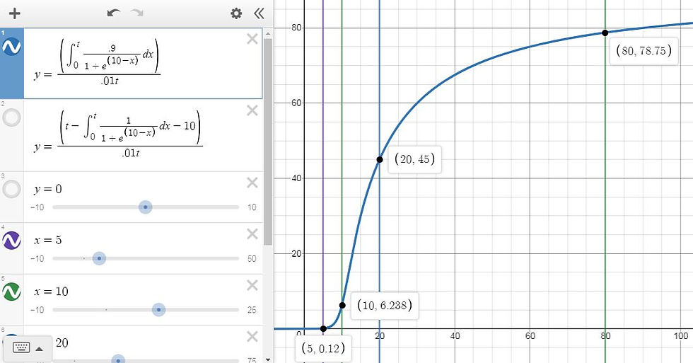
To find the actual tax rate, I divided tax amount by pretax income, giving this curve (the y-axis is in units of percent):

Subtracting tax amount from income shows actual amounts kept after tax:

At low incomes, like above, a dollar earned is at most a dollar earned after tax. At high incomes, like below, a dollar earned is at least ten cents earned after tax.

---------------------------------

There is a point where a household can afford everything it needs. Before that point, no money should be taken unless the government produces more value for the household from that tax revenue than the household itself can do. Past that point, a greater and greater amount of income should be taken. The government can likely produce more value for society than the household itself, through projects like education subsidies, sovereign wealth funds, or infrastructure spending. However, those are articles for another time.

Thank you for reading,

George Fane

See this tax system's combination with a Negative Income Tax.