Polynomial Integrator

Maybe a week or two ago, I was wondering how to make a program that would output eigenvalues for an inputted matrix. To do that, I would need to know how to find x-intercepts given a polynomial (the determinant of the inputted matrix minus lambda times the identity matrix). I didn’t figure it out, but during my search that day I read about the roots function in MATLAB, which intakes a vector containing the coefficients of the polynomial whose roots are desired to be found.

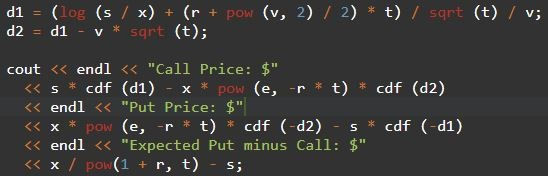
That got me thinking about making a polynomial integration program. I had learned about the Monte Carlo method for integration a few weeks before for my second option valuation program, and this new-to-me concept of storing coefficients in a vector would help me record info about the polynomial to be integrated.

Program

https://repl.it/@GeorgeFane/polynomial-integrator

Polynomial Integrator - Sample Output

My original plan was to have the program user input their polynomial’s highest and lowest exponents and prompt the user for every coefficient between those two values, perhaps requiring the user to input several zeroes for terms that aren’t there (under this strategy, for example, x ^ 9 - 1 would require eight zeroes to be entered between 1 for the first term and -1 for the last term). This is similar to how MATLAB does it, treating the vector’s rightmost value as the coefficient of x ^ 0 and treating every value to the left as the coefficient of successively higher-exponent terms. The vector sometimes needs a few zeroes.

I switched to a loop that would ask for each term’s coefficient and exponent in that order, going on forever (the loop heading says while True:) until 0 is entered for a coefficient. To do that I made my ‘coefficient vector’ a list with two rows, the top storing coefficients and the bottom storing exponents.

I should’ve split the two-rowed list into two different lists, each with a more descriptive name than the current terms, but I wanted to make sure both lists were properly aligned when iterated through for the integration algorithm. This was a stupid reason, because if I used two separate lists both would’ve had the same length anyways. I also did a little research while writing this article and found the zip() function that would’ve let me iterate through two different lists at the same time with a for each loop.

The integration algorithm starts similarly to the one in Black-Scholes Revisited, with a for loop with the range of some relatively high number. A new random number or x-value is generated for each iteration and is run through an embedded for loop that calculates that x-value to the power of an exponent in the terms list times the corresponding coefficient. This is done for each term in the polynomial and added up to produce one final y-value for every x. All y-values are then added up in the variable add. The last step is to show the value of the polynomial’s definite integral, which needs add to be divided by the number of random x-values and multiplied by the distance between the integral’s upper and lower bounds.

After I completed the aforementioned code, I realized that I wanted to display the polynomial nicely after the user entered all coefficients and exponents. I didn’t want to merely print both lists, so after each term had its two coefficient and exponent entered, the string poly would have that new term, nicely formatted, concatenated to it. This string-building takes place in the same for loop that prompts the user for coefficients and exponents.

I learned a lot about string formatting for this program. Not long before, I exclusively used commas to separate normal strings and variables inside print functions, bemoaning the seemingly-unavoidable space in the output that came with each comma. Using %s or %f, say, in my print functions helps me keep track of all spacing that’ll show up in the output and help me show those variable values in very customizable ways. For a while I formatted the coefficient as %+.2f when constructing the poly string, because I needed the format to be a float (%f) in case the user entered a coefficient with decimals, I wanted the displayed float to not take up too much space (without the .2, %f often has a long chain of useless zeroes to the right), and I needed the + sign to show up between terms. Otherwise, ‘this term plus that term’ would have the ‘plus’ missing.

I also made a long series of if statements to not show the power sign if the exponent was 1 or 0, and to not show the coefficient if it was 1 or -1. My brain was super slow at the time, so figuring out the special cases of showing the coefficient no matter what if the exponent was 0 and showing the x but not the power sign if the exponent was one was a pain. It was weird. Writing it out here makes it seem so simple.

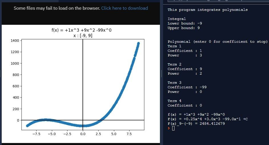
In the end I simplified the poly string-building to %sx^%s, with the coefficient and exponent cast to strings. The entered digits would be shown - no more, no less. If the coefficient was positive, the plus sign would be added to the beginning. This simple process leads to ugly displays best exemplified by the string +1x^0 -1x^1, when humans would just write 1 - x.

I also created the inte string that would display the original polynomial’s integrated form. In the same for loop that prompts the user for terms and builds the poly string, the inte string adds on %sx^%s for each term, just like poly. The first %s represents the inputted coefficient divided by power plus one when cast to string, and the latter represents power plus one, in accordance to the rules when integrating polynomials. If the term has a power of -1, then inte instead adds coefficient times the natural log of x’s absolute value, cast to string.

Finally, I wrote into the code the ability to graph the randomly selected x and y-values. When seeing the graph the first few times, I realized that I made a mistake in the for loops that performed the Monte Carlo integration. I put the random number generator inside the interior for loop, which meant that as the loop iterated through the terms of the polynomial, a different x was used each time. Also inside that interior for loop, I added the value of every term to ylist, which I would later graph. These two mistakes put together meant that a three-termed polynomial would produce three different curves on the plot Polynomial Graph.png.

The initially surprising result was that the definite integral’s value was still accurate. Thinking it over later, though, choosing a random value to plug into each term and getting the right result makes as much sense as choosing a random value and putting it into every term each iteration and getting the right result. The latter is the typical method of approaching Monte Carlo integration, but such a method teaches us that choosing a high enough number of random inputs offers a reliable output. By that I mean that with so many points on each of the multiple curves, there must’ve been a randomly-generated x-value on the first curve that was pretty close to one on the second, third, and nth curves. The corresponding y-values on each of the curves, added up, most probably equaled the whole polynomial’s value given a single x-value, which, when done many, many times, is what the Monte Carlo method is all about.

Another way to approach the integral's correctness despite several different x-values is much simpler and came to me while writing this article. The integral of a polynomial can be split into the sum of the integrals of each term. By using a different x for each term, it’s like I was performing a Monte Carlo integration on each term separately and adding up the totals for each. My supposed mistake of inputting a random x into each term actually still works, even if I didn’t realize it. Also, it was faster than my current system.

But all of those two previous paragraphs didn’t matter because I wanted a nice plot of the inputted polynomial, which required me to use a single x for all terms to plot against a single y each iteration. I added an x-axis and y-axis using axhline and axvline, and set the plot’s title as the string poly along with the bounds of integration/x-value generation. I didn’t know that such labels could contain variables before writing this part of the program. As the cliche goes, you learn a new thing every day. As most people know, it’s often several things.

---

I set out to merely intake a polynomial along with bounds and return the definite integral’s value. I ended up with, other than the aforementioned, a polynomial displayer, a polynomial indefinite integral displayer, and a polynomial grapher. Along the way I learned more about string formatting, which will definitely make my future programming easier and more customizable. This stay-at-home order has not always been enjoyable, even though I recognize its vital importance in keeping Michiganders safe, but at least I have these programs to work on and learn from.

Thank you for reading!

George Fane