Revisiting Black-Scholes

At the end of February, I started going on the Corporate Finance Institute website again. It offered new certifications with new video series, so I started watching "Introduction to Derivatives". I saw option payoff diagrams for the first time in half a year and remembered how I wanted to build my own when I first made my option valuation programs. This time, I knew I could if I just learned a bit more about the Matplotlib library for Python.

It took a while to find a good interpreter for my needs. OnlineGDB, my usual choice for programming, doesn't seem to have libraries. I thought of using offline IDEs but didn't think I could embed their code and outputs into this website. Finally, I found Repl.it, which has multiple Python libraries already installed while also handling multiple languages, like OnlineGDB. The only thing is that Repl.it is noticeably slower at running code, but still, it is better on the balance.

Program

https://repl.it/@GeorgeFane/Visual-Black-Scholes

This program has multiple differences from the original, starting with the language: this is in Python, while the other is in C++.

OOP

The second is the use of objects. The older C++ program did nearly every calculation in the main function, in a rather ugly way as I’m looking back now:

Keeping that in mind, I created the Option class whose objects would store the Black-Scholes Formula’s five inputs. That way I don’t need to pass those five inputs as parameters over and over again to my d1, d2, call price, and put price methods.

We hadn’t actually learned about classes and objects in Python during CompSci Principles, but we did in Java for CompSci A, so that knowledge transferred over rather well. Python’s rather similar process still held surprises: the __init__ function is used to define objects, rather than writing a public (name of object) method. Also, the self parameter must be passed to every method within a class to access the object’s private variables. However, one nice thing is that I don’t need to write get methods to access those variables in the main function; I can refer to them directly as I did near the very bottom of the code:

CDF

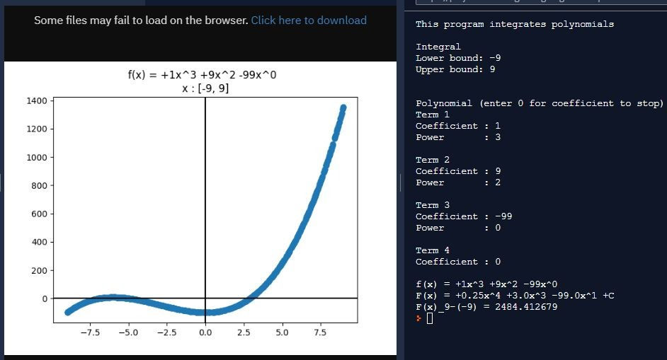
The third difference is in calculating the cumulative distribution function. I was determined to use Monte Carlo integration, which averages several randomly-chosen areas along a curve, as a change of pace compared to my original Taylor series strategy. That series was hard to come up with at first, but since then I’ve been able to recall it easily. Monte Carlo would pose a new challenge.

The above image helped a great deal in my understanding of Monte Carlo integration. A few crude “areas under the curve” can be found by multiplying the width of the definite integral trying to be found by random heights. Some areas will be too small and some will be too large, but averaging them should give a decent, more accurate answer in the middle. As more and more areas are included, this method of integration becomes more accurate.

In my program, I first add up several random heights, not areas, and only multiply by width after I’ve averaged those heights. I also treat PDF(-3) as zero and thereby treat CDF(x) as the definite integral of PDF from -3 to x.

I’d say the Taylor series is better because it gives the same answer every time, and with only a ninth degree expansion gave answers that lined up very well with online CDF calculators. This Monte Carlo integration generates 999 random heights, which takes especially long in Python compared to running a C++ Taylor series, and outputs different values for the same input when used multiple times.

Because each calculation of call and put price (getCall() and getPut()) runs the CDF function twice each, I only use those get functions once each and store their returned value in a private variable in the __init__ function.

Charts

The most significant difference, as well as the most visible, is the charts. Creating those payoff diagrams was the reason I made a new version of my option valuation program.

The first one I made, though, was in the ‘Standard Normal Distribution.png’ file (you can find it by clicking the document icon in the program's top left). At the time, my CDF function was just awful, giving completely wrong answers. I wanted a way to qualitatively check whether the function’s outputs made sense for their inputs, d1 and d2, so I plotted those two values as vertical lines (axvline). I also controlled the domain and range of the graph using the axis function to show the typical width of a standard normal distribution curve, even if not all of the curve is shown every time. Normally, though, I don’t set axis and let Pyplot handle the sizing automatically, like I allow below.

For the very similar callPayoff() and putPayoff() functions, which create the corresponding payoff diagrams, I actually changed them significantly while writing this article. Originally, I created a profit function for each of the two diagram creators. For call options, it was max (x - self.strike, 0) - self.call, where x is a randomly chosen underlying asset price. I would run that profit function several dozen times using a for loop and add each randomly chosen x to a list called xset and add the profit function’s ouptut for each x to a list called yset. After that, I’d sort both xset and yset from smallest to largest and run plot (xset, yset).

As I looked at that code though, I realized that I could simply plot three points: the leftmost point, the rightmost point, and the point in the middle where the slope changes. Those three points define two line segments, one of which would be flat with a y-value equal to the cost of the option, representing the situation where it is less profitable to exercise the option than to let it expire. The second, sloping line segment represents the other scenario, where underlying asset price is either relatively high to be useful for a call option, or relatively low for a put.

After that, I added three vertical lines for strike price, spot price, and break-even price, color-coded identically between the two charts. With that, I had developed a new version of my option-pricing program that included the visual aid of payoff diagrams.

---

Learning more about math, programming, and finance: what's not to love? It was a good idea to go back to that CFI website again; that drove me to create my first few finance programs, including the one involving options, and it has brought me back again to that topic. Options don't stop at this article, though. I'm trying to develop a program displaying the volatility smile, a graph comparing strike price and implied volatility. An article on that is upcoming, once I figure out how to make it. :)

Thank you for reading!

George Fane