Black-Scholes Option Valuation and Implied Volatility
- George Fane

- Aug 28, 2019
- 3 min read
Updated: Apr 6, 2020
I probably first saw the Black-Scholes Formula for option valuation a few weeks ago. I had just finished up the CFI's video series on bonds and corporate finance and started to look for other free sources of finance education. I found the videos on the Black-Scholes Formula and Implied Volatility on Khan Academy but had trouble thinking up code for a cumulative distribution function. However, with my CDF program out of the way a few weeks later, I was ready to begin my Black-Scholes Formula program.
Black-Scholes Formula
Your first time looking at the formula, you will be slammed by an incomprehensible multitude of natural logs and N() functions. If we break it down, though, the formula can become understandable. An option is the ability to buy or sell some share in the future at a certain price. Because share prices can move very unpredictably, an option reduces risk. Therefore, it is valuable and must have a price itself.
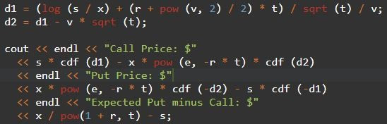
For a "call" option, which guarantees that a share can be bought at a certain price in the future (as opposed to a "put" option, guaranteeing a sale), the option C is essentially worth current price S (spot price) minus the future buy price X (strike price or exercise price). This means that valuable options allow the purchase of expensive shares at low prices:

Strike price, occurring in the future, has a higher nominal value at the maturity date compared to real value today, so it must be discounted:

where r is risk-free rate of return in percent per year and t is years until the option's expiration.
Each of the terms on the right side of the equation are then multiplied by cumulative distribution functions N(d) that together return the probability that spot price exceeds discounted strike price:

where v is volatility of share price.
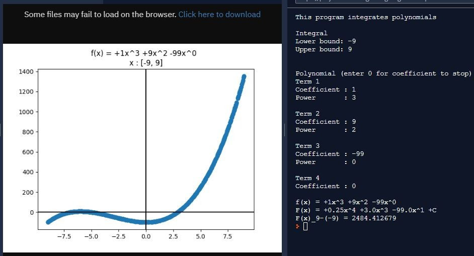
As I mentioned in the SNCDF Article, standard C++ cannot perform integrals or work with infinitesimals; a Taylor Series approximation may not be perfectly accurate but is a strong runner-up:

Note: I used a 9th degree approximation, so the inf above the final Sigma would be a 9 in my final program.
Put option valuation is very similar to that of call. The seller wants to execute a sale for more money than the current price, so the formula is essentially reversed:


Creating a CDF program was definitely the hardest part of this whole process. I converted Program CDF's int main() into a function in Program Black-Scholes, then copied over the factorial function. From there, I had the simple task of outputting prompts for the user to enter values, and sticking said values into the Black-Scholes Formula.
However, I soon had another challenge: given the option value and most of the Black-Scholes Formula's inputs, calculate volatility.
Implied Volatility
Looking at the equation for option value, volatility cannot be solved for as far as I can tell. It likely requires the variable for volatility to be separated from the others in the d1 and d2 equations. After that, a method to get a CDF's input given its output must be known, which I have not learned. Instead of solving for volatility, perhaps smart guess-and-check should be used.

This program is rightfully very similar to Program Black-Scholes; all I need to do is randomly generate volatility values. Of course, the generation is not truly random; as I mentioned in the NPV and IRR article, I start at some arbitrary volatility, use it to calculate a call price, and jump back and forth over the inputted call price by smaller and smaller amounts until the call price linked with my volatility has a small enough difference from the input:

This approximation system is more complicated and less functional than that in Program IRR. I essentially set a maximum value and starting point of 200% volatility and a minimum value of 0% (unfortunately, this appears to cap the maximum implied volatility at 400%). Depending on whether the calculated option price was higher or lower than the input, the upper or lower volatility bound would get closer to the other by half the distance between the bounds.
Just building that code was difficult, but once my program began to work, I noticed that some call prices could have two different volatilities:

I inputted random values for the first Black-Scholes calculation (including a 9% volatility), took the call price of $3.5 and ran it through my Implied Volatility program, then took the outputted volatility of roughly 14.5% and ran it through my Black-Scholes program again. As you can see, volatility changes between the first and second calculations but call price barely does.
Building the Black-Scholes and Implied Volatility programs were enjoyable challenges. In both cases, I used advanced math that I had not encountered for months (integrated power series for the former and convergent alternating series for the latter), and had to break down these programs into smaller, more manageable pieces. By forcing me to create and apply complex processes, developing these calculations furthered my understanding of finance.
Thank you for reading!
George Fane

Comments